Everybody talks streaming nowadays – social networks, online transactional systems they all generate data. Data collection means nothing without proper and on-time analysis. In this new data age, we are privileged with the right tools to make the best use of our data. We can use structured streaming to take advantage of this and act quickly upon new trends, this could bring to insights unseen before.

Spark offers two ways of streaming:
• Spark Streaming
• Structured streaming (officially introduced with Spark 2.0, production-ready with Spark 2.2)

Let’s add a few words for both streaming options below.

Spark Streaming

Spark Streaming is a separate library in Spark which provides a basic abstraction layer called Discretized Stream or DStream, it processes continuously flowing streaming data by breaking it up into discrete chunks. DStream is the original, RDD (Resilient Distributed Dataset) based streaming API for Spark.

Spark streaming has the following problems:
• Difficult – not simple to build streaming pipelines which support late data or fault tolerance. All of them are achievable but they need some extra development work.
• Inconsistent Integration- API used to generate batch processing (RDD, Dataset) is different than the API of streaming processing (DStream).
• Processing order – later generated data is processed before earlier generated data.

Structured Streaming

Structured streaming is based on Dataframe and Dataset APIs, it is easier to implement and SQL queries are easily applied. Most importantly, Structured streaming incorporates the following features:
• Strong guarantees about consistency with batch jobs – the engine uploads the data as a sequential stream.
• Transactional integration with storage systems – transactional updates are part of the core API now, once data is processed it is only being updated, this provides a consistent snapshot of the data.
• Tight integration with the rest of Spark – Structured Streaming supports serving interactive queries on streaming state with Spark SQL and JDBC, and integrates with MLlib.
• Late data support – explicit support of “event time” to aggregate out of order data (late data) and bigger support for windowing and sessions, this avoids the problems Spark Streaming has with Processing Order.

Structured Streaming example

In this blog, we will focus on the basics of structured streaming. We will demonstrate some simple visualisations of streaming data used to validate if the stream worked.

Source Data

For this tutorial I’ve used open-source data for taxis in NYC:

https://www1.nyc.gov/site/tlc/about/tlc-trip-record-data.page

The purpose of this blog is to introduce you to structured streaming using a simple scenario with CSV input data with specific dates and times which we will be able to use. The static set of files are used to emulate streaming taxi orders. I computed real-time metrics like peak time of taxi pickups and drop-offs, most popular boroughs for taxi demand.

In order not to overload the Databricks cluster, I took one FHV Taxi CSV file – for January 2018 and split it into multiple smaller sized files.

The data is 11 CSV files – 10 with transactional records and one location mapping, each transactional CSV file has about 5000 rows. The collection of the files serve as an echo of what real data might be like.

I’ve done some testing in terms of storage – if you decide to use ADLS the structured streaming won’t be working since it requires uploading of new files in the streaming folder or editing while the streaming is on. 

For the below exercise I chose DBFS as a storage location.

All source files and Databricks notebook can be found on the following link:

https://github.com/VickyAugust10/PysparkStructuredStreaming

Shall we get started?

Let’s get a preview of our main source folder:

%fs ls "/FileStore/tables/streaming/"

Now let’s check how our CSV files look like, they are all the same in terms of structure:

%fs head "/FileStore/tables/streaming/fhv_tripdata_2018_01_1-b3a55.csv"

And lastly we need to make sure our location file contains Borough and zone names and codes:

%fs head "/FileStore/tables/streaming/Lookup/NYC_Taxi_zones.csv"

Data Loading

Let’s investigate the static data first by creating a data frame and naming it staticInputDF. Only the first 4 columns are required for our analysis, hence only these have been selected.

from pyspark.sql.functions import * 
from pyspark.sql.types import *

inputPath = "/FileStore/tables/streaming/"

staticDataFrame = spark.read.format("csv")\
   .option("header", "true")\
   .option("inferSchema","true") \
   .load(inputPath) \
   .select("Pickup_DateTime", "DropOff_datetime", "PUlocationID", "DOlocationID")

OrderSchema = staticDataFrame.schema 
display(staticDataFrame)

Now let’s load the mapping table for NYC zone and borough names:

LocationPath = "/FileStore/tables/streaming/Lookup/NYC_Taxi_zones.csv"
df_Location = spark.read.option("header", "true").csv(LocationPath)

display(df_Location)

Let’s add some business logic for the purposes of the analysis, we need to combine Pickup_datetime and Dropoff_Datetime in one column – called ServiceTime and adding a new hardcoded column for Service Type. We also need to join our static data frame with the location mapping table to retrieve the borough and zone names.

df_Pickup = staticDataFrame.select(col("Pickup_Datetime").alias("ServiceTime"), col("PUlocationID").alias("Location")).withColumn("ServiceType",lit("Pickup"))
df_Dropoff = staticDataFrame.select(col("Dropoff_Datetime").alias("ServiceTime"), col("DOlocationID").alias("Location")).withColumn("ServiceType",lit("DropOff"))

df_final = df_Pickup.union(df_Dropoff)
df_final = df_final.join(df_Location,df_final.Location == df_Location.LocationID, 'left' ).withColumn("ServiceHour", hour("ServiceTime"))

df_final.createOrReplaceTempView("taxi_data")
staticSchema= df_final.schema

display(df_final)

Now we can compute the number of “Pickup” and “Dropoff” orders per borough, Service hour, Service day with one-hour windows. To do this, we will group by the ServiceType, ServiceHour, ServiceDay and borough columns and 1-hour windows over the Servicetime column.

from pyspark.sql.functions import *      # for window() function

staticCountsDF = (
    df_final\
      .selectExpr( "Borough",
                   "ServiceType",
                   "ServiceHour",
                   "ServiceTime").withColumn("Service_Day",  date_format(col("ServiceTime"),'EEEE'))
        .groupBy(
                     col("Service_Day"),
                     col("ServiceType"),
                     col("ServiceHour"),
                     col("Borough"), 
                     window("ServiceTime", "1 hour")) 
                .count()
            )
 
staticCountsDF.cache()

# Register the DataFrame as view 'static_counts'
staticCountsDF.createOrReplaceTempView("static_counts")

Now we can directly use SQL to query the view. For example, here are we show a timeline of windowed counts separated by Service type and Service hour.

%sql
select ServiceType,Servicehour, sum(count) as total_count from static_counts group by ServiceType,Servicehour order by Servicehour, ServiceType

How about checking the count of pick up orders made in different boroughs per day? Most pick up orders have been registered in Manhattan, Brooklyn and probably online in the cases where borough is blank?

This is not a surprise, is it?

%sql
select Borough,Service_Day, sum(count) as total_count from static_counts where Servicetype = 'Pickup' group by Borough, Service_Day order by Service_Day

Structured Streaming processing

Now let’s convert our static query into a steaming one, which constantly updates as data arrives. Both queries are very similar and the main key difference is that instead of .read we use .readstream.Since we are using a static set of files, we are going to read one at a time.

from pyspark.sql.types import *
from pyspark.sql.functions import *  

spark.conf.set("spark.sql.shuffle.partitions", "2") 

streamingDataframe = (
  spark
    .readStream
    .schema(OrderSchema)
    .option("maxFilesPerTrigger", 1) \
    .format("csv")\
    .option("header", "true")\
    .load(inputPath)
)

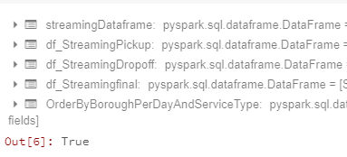
Let’s add the same logic as before. The result of the last command OrderByBoroughPerDayAndServiceType.isStreaming is true, meaning our streaming is active.

# Let's add some business logic
df_StreamingPickup = streamingDataframe.select(col("Pickup_Datetime").alias("ServiceTime"), col("PUlocationID").alias("Location")).withColumn("ServiceType",lit("Pickup"))
df_StreamingDropoff = streamingDataframe.select(col("Dropoff_Datetime").alias("ServiceTime"), col("DOlocationID").alias("Location")).withColumn("ServiceType",lit("DropOff"))
df_Streamingfinal = df_StreamingPickup.union(df_StreamingDropoff)

# Join Streaming data with location mapping table to retrieve the relevant NYC zone names
df_Streamingfinal = df_Streamingfinal.join(df_Location,df_Streamingfinal.Location == df_Location.LocationID, 'left' ).withColumn("ServiceHour", hour("ServiceTime"))

# Same query as staticInputDF
OrderByBoroughPerDayAndServiceType = (                 
  df_Streamingfinal
   .groupBy(
     date_format(col("ServiceTime"),'EEEE').alias("Service_Day"),
       df_Streamingfinal.ServiceType,
       df_Streamingfinal.ServiceHour,
       df_Streamingfinal.borough,
       window(df_Streamingfinal.ServiceTime, "1 hour")
          ) 
    .count()
)

OrderByBoroughPerDayAndServiceType.isStreaming

Now we have a streaming dataframe, but it is not writing anywhere. We need to stream to a certain destination using writestream() on our dataframe with concrete options:

spark.conf.set("spark.sql.shuffle.partitions", "2") 

query = (
  OrderByBoroughPerDayAndServiceType
    .writeStream
    .format("memory")        # memory = store in-memory table (for testing only in Spark 2.0)
    .queryName("counts")     # counts = name of the in-memory table            
    .outputMode("complete")  # complete = all the counts should be in the table
    .start()
)

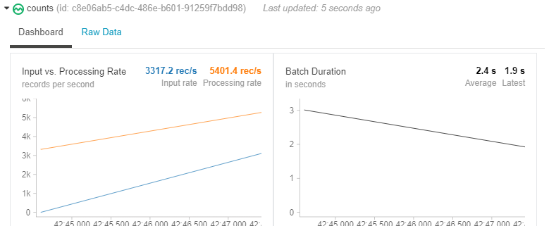
We can now watch the data streaming live while in our notebook.

Let’s wait 5 seconds for some data to be processed:

from time import sleep
sleep(5)

Let display the same charts as we did for our static data:

%sql
select ServiceType,Servicehour, sum(count) as total_count from counts group by ServiceType,Servicehour order by Servicehour, ServiceType

%sql select Service_Day, borough, sum(count) as total_count from counts group by Service_Day, borough

 

Let’s pause the streaming for 5 seconds and move our “new” files from NewTripsData folder to the streaming location.

Please have a closer look, you can notice that the total counts – for the first bar jumped from 12k to above 20k and for the second chart from a bit above 30k to above 35K. Also, the trends slightly changed – the difference in the pickups between 16 and 17 is much bigger now. Manhattan kept the first place for most popular pickup location. Have in mind this data represents just a few January days, and for some reason, people were most active on Wednesdays.

sleep(5)

%sql
select ServiceType,Servicehour, sum(count) as total_count from counts group by ServiceType,Servicehour order by Servicehour, ServiceType

 

%sql select Service_Day, borough, sum(count) as total_count from counts group by Service_Day, borough

 

This concludes our first encounter with Pyspark structured streaming, I can definitely think of many cases where it can be applied.

Please let me know your feedback, any suggestions and comments are very welcome, get in touch!

Till next time!