How often do you find yourself in a situation where people are talking about statistics and you can’t way in because you’ve forgotten everything from school and univeristy?

Well, no more! ????

We are going to go through some basic statistic concepts that are commonly used for data exploration/analysis/sciency stuff.

We will discuss the normal distribution, some statistical features, visualisations of statistical features and for next time – the almighty Bayes.

Let’s dive in!

Normal Distribution (a.k.a. Gaussian distribution or Bell curve)

The Normal Distribution is used to represent real-valued random variables whose distributions are not known.

It is common distribution we encounter when working with various types of data used in the natural and social sciences.

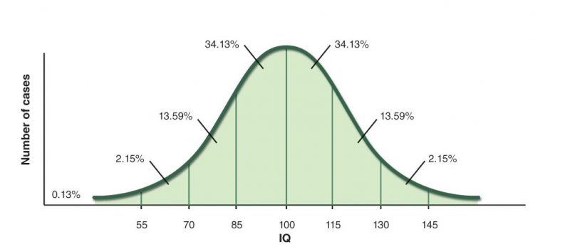
For example the height of people, the blood pressure, errors in measurements, IQ scores – all these very closely resemble the normal distribution

What is the reason behind the natural occurance of this distribution?

The answer lies in the Central Limit Theorem – basically it states that the average of many samples (observations) of a random variable with finite mean and variance is itself a random variable whose distribution converges to a normal distribution as the number of samples increases. In other words if you have enough records of a random variable it’s sample average distribution converges to normal distribution even though the variable’s distribution itself might not be normal. This also means that any variable that is result of the combination of many effects will be approximately normal.

//The CLT also means that any variable that we measure that is the result of combining many effects (many relative to the degree of relationship between the different pieces) will be approximately normal

Consider the annual rainfall for a certain area, even though the daily rainfall most likely would not be “normal”, the sum of all observations per day would result in a distribution close to the normal.

There are certain random processes that produce normal distribution as well. Check out the quincunx for example.

Even though many accurate and often more precise distributions exist, the normal distribution is (still) widely used in predictive analysis and hypothesis testing.

Why – mainly because it is simple to understand. It only uses two parameters and many otherwise complicated mathematical operations on the data are made simpler if the assumption of normality is present.

Also it offers a gentle introduction to the world of distributions and is therefore essential to introductory statistics courses.

But for me normal distr. in the world of statistics is like the regression in ml world – yes, there are better, more precise methods but they are also more complicated to perform (and to understand – a factor not to be dismatched, you don’t need a degree in mathematics to understand these simpler concepts which is not always the case when things get more coplex). How often in real life solutions for real life bisunesses (that are not NASA) you get to use neural networks to predict something, and how often the good old regression does the job?

The general form of the probability density function of the normal distribution is:

If we display all possible values of our random variable (for the IQ example those would be all scores between 55 and 145 roughly) the prob.density function would give us the relative likelyhood that our ranodom variable (IQ score) equals any of the possible values.

There are two parameters here: ???? and ???? where ???? is the mean (and in this case also the median and the mode) – the probabilistic version of arithmetic mean and a measure of central tendency of the distribution; the second parameter – ???? – is the standard deviation – a measure of the amount of variation or dispersion of a set of values. A low standard deviation indicates that the values tend to be close to the mean of the set, while a high standard deviation indicates that the values are spread out over a wider range.

If we square the standard devaition we get the variance of a distribution – how far our set is spread out from the average value (the mean value).

I mentioned some other statistical features so let’s define them as well:

• arithmetic mean (mathematical expectation, average) is the sum of values divided by the number of values
• median is the value separating the higher half from the lower half of a data sample in other words the value exactly in the middle of the set
• mode is the value that appears most often in a set

Knowing that let’s take another look at the bell curve and place those features on the plot:

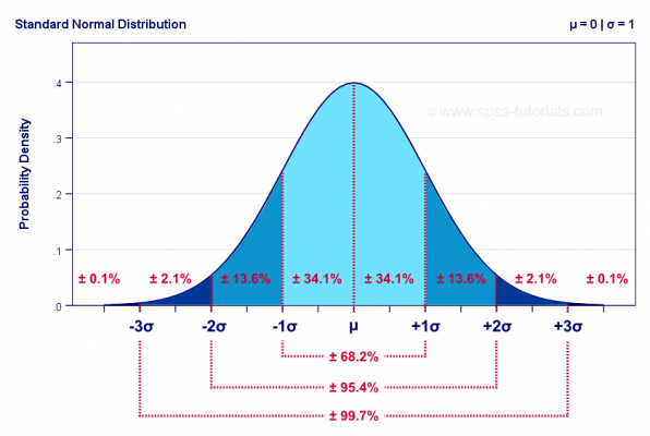
The mean (????) is the value corresponding to the highest probability density. The bright blue part of the plot shows that 68.2% of the data is located within one standard deviation away from the middle in each direction.

As we get further away from the mean we get less and less observations. If we look at the IQ chart again we see that the people with IQ higher that 130 are only around 2% of the population i.e. the probability that you are really really smart (assuming that you are a random person) is only 2%.

We just used another stats feature – percentile – the measure indicating the value below which a given percentage of observations in a group of observations falls.

Now that we have revised some basic statistic features we might want to visualize them.

Boxplots are a great way to do this. They show the basics and give a quick overview of the distribution of the data.

This is a boxplot of normally distributed data:

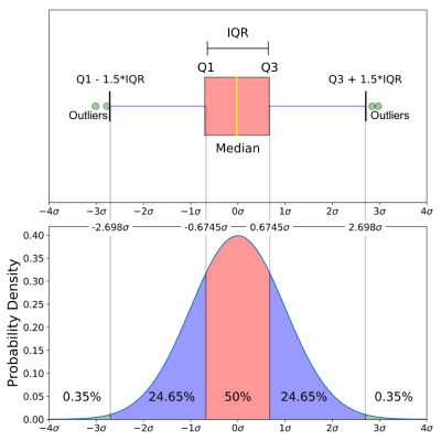
Let’s go through the plot – the yellow line – the median – we are already familiar, the Qs are the percentiles: Q1- the 25th percentile, Q3- the 75th, meaning that the body of the boxplot represents 50% of the data; We have min and max which is (almost) our lowest and highest values. The outliers – the extreme low or high values in our data. The purple lines are called whiskers. The IQR (Interquartile range) is simply Q3 – Q1 and determines what will be the min/max values and the outliers.

Not all boxplots will look as pretty and symmetrical. Depending on the distribution of the data we might get something like this:

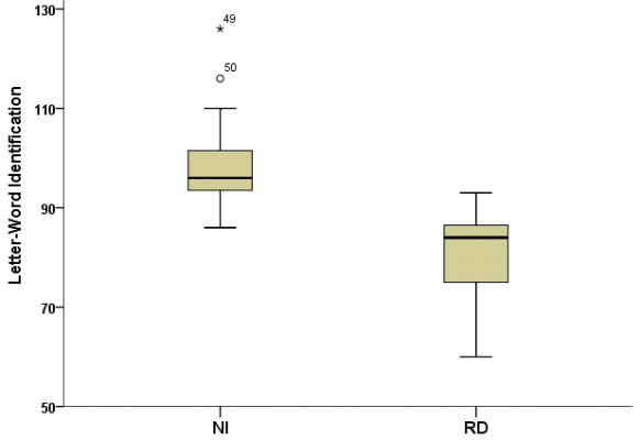
If the data is skewed some direction that means most records are close to the min/max. If the whiskers are long then the data is more spread out, if the median is close to the min/max then half the data is close to this value, if the “body” is tall then the data is more sparse, if the body is short then the data is more close etc.

Now that we have covered some basics around the distribution of our data, let’s talk about the content. Usually we work with tabular data with some attributes (columns) and the relations between them can give us valuable insights on how the process we observe works. There is a metric for calculation the dependence between two variables – the correlation coeficient. Mathematically this is the covariance(the joint variability of two variables) devided by their standard deviations.

ρ(????,????)=????????????(????,????)/????????????????

The correlations between all attributes are usually displayed as a matrix. This gives a good overview and is sometimes used as a step in feature selection for model building.

 

 

 

This concludes our very brief overview.

To demonstrate the use of statistics in some basic data exploration i am using the public dataset provided by kaggle.com. The references for the data can be found below.

The entire code is available here. — add link to github !!!

 

 

Data References

United Nations Development Program. (2018). Human development index (HDI). Retrieved from http://hdr.undp.org/en/indicators/137506

World Bank. (2018). World development indicators: GDP (current US$) by country:1985 to 2016. Retrieved from http://databank.worldbank.org/data/source/world-development-indicators#

[Szamil]. (2017). Suicide in the Twenty-First Century [dataset]. Retrieved from https://www.kaggle.com/szamil/suicide-in-the-twenty-first-century/notebook

World Health Organization. (2018). Suicide prevention. Retrieved from http://www.who.int/mental_health/suicide-prevention/en/