This is where the real fun begins! In this blog we will get to the heart of machine learning and produce a regression model.
Training the model
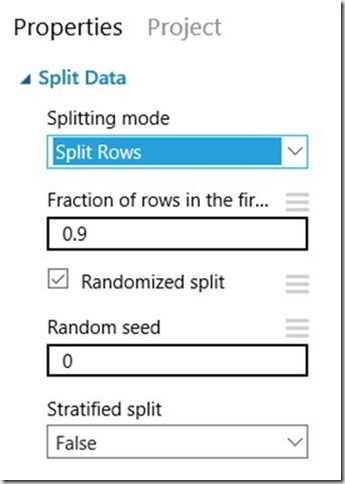
We now need to split the data into training and testing sets. This is so we can train the algorithm using the training set and then test the accuracy of the prediction using the testing set. To do so search for ‘split‘ in the Search experiment items search bar. Drag the Split Data task onto the canvas. Under the properties is a property called Fraction of rows in the first output dataset this lets you chose what percentage of rows is used for training and what percentage are held back to test the prediction accuracy. Let’s set it to 0.9, this means 90% will be used for training, 10% for testing. Leave the other properties as they are. The properties window should look like the below image:
Now let’s get to the very fundamental core of machine learning, the algorithm itself. For this we will use one of my personal favourites a Boosted Decision Tree. Decision Trees frequently have very high accurate prediction results and are great for discovering more about your data based on the leaves of the tree. Go to the item toolbox, clear the search box and navigate to Machine Learning > Initialize Model > Regression and drag on the Boosted Decision Tree Regression item onto the left side of the canvas. Change the properties to coincide with the values below, these have been selected after using a Sweep Parameters item to work out the optimal parameter settings.
| Parameter Name | Parameter Value |
| Create trainer mode | Single Parameter |
| Maximum number of leaves per tree | 36 |
| Minimum number of samples per leaf mode | 7 |
| Learning rate | 0.33128 |
| Total number of trees constructed | 182 |
| Random number seed | |
| Allow unknown categorical levels | Check |
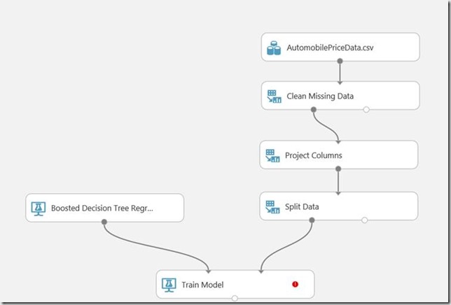
Drag on the Train Model item, which is located under Train on the item toolbox. Join up the appropriate output and input ports so your canvas looks like the image below.
Click on the Train Model item and select Launch column selector in the properties window. Here you are selecting the column you want to predict, so just select price.
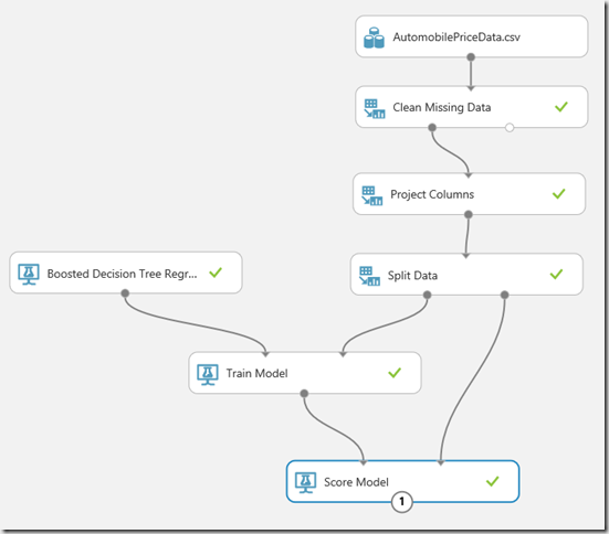
Now we need to predict the results of the testing data. To do so, drag on a Score Model item (located under Score) and connect the Train Model and Split Data items to each input note of the Score Model. Once complete, hit Run to run the experiment, your canvas should be eliminated with green ticks like the image below.
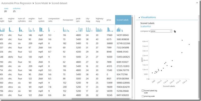
Now let’s have a look and see if this algorithm has actually produced any decent results. Right click on destination node of the Score Model and left click on Visualise. You should see something similar to the below image.
This table displays the values for each and every piece of test data. If you scroll all the way to the right and you should see two columns: price and Scored Labels. Price is the actual price of the car. Scored Labels is the amount the regression algorithm has predicted the price of the car to be. The numbers are quite close, which is exactly the result we’re after. If you click on the Score Labels column header you can conduct some further analysis, scrolling down and making sure compare to is set to price you can view a scatter plot of the two values. I have done so on the image above and looking at the scatter plot you can see that there is a strong positive correlation with only a few outliers.
Your Azure Machine Learning regression algorithm is now complete! In the next blog we will be deploying the model so we can use it outside of Azure Machine Learning and really put what we have created into practice.


